TL;DR
Modern speech-synthesis systems leave subtle high-frequency (HF) artifacts that frequency-agnostic detectors ignore — a manifestation of spectral bias. SONAR is a dual-path detector that fuses an XLSR content branch with a parallel branch driven by learnable, value-constrained SRM high-pass filters, and trains them with a Jensen–Shannon alignment loss that pulls genuine LF/HF representations together while pushing fake ones apart. SONAR achieves state-of-the-art performance on ASVspoof 2021 and In-the-Wild, converges 4× faster than strong baselines, and degrades gracefully under codecs and bandwidth shifts.
Motivation
Generative voice cloning is now cheap, fast, and convincing. The 2024–2025 election cycle brought a wave of political audio deepfakes; voice-cloning fraud has caused multi-million-dollar losses at corporations and call-centres. Yet most existing detectors collapse the moment they see a generator they were not trained on — a generalisation failure rather than a capacity one.
The pattern they share: networks fit low-frequency structure first and under-utilise the subtle high-frequency residuals where vocoders leave their fingerprints (the frequency principle). Real and synthetic speech differ not only in marginal HF energy, but in the joint LF–HF consistency of the signal — a relationship that frequency-agnostic detectors systematically miss. SONAR is built around this observation: instead of treating HF residuals as auxiliary features or aggregating them late, we couple them to semantic content during training itself.
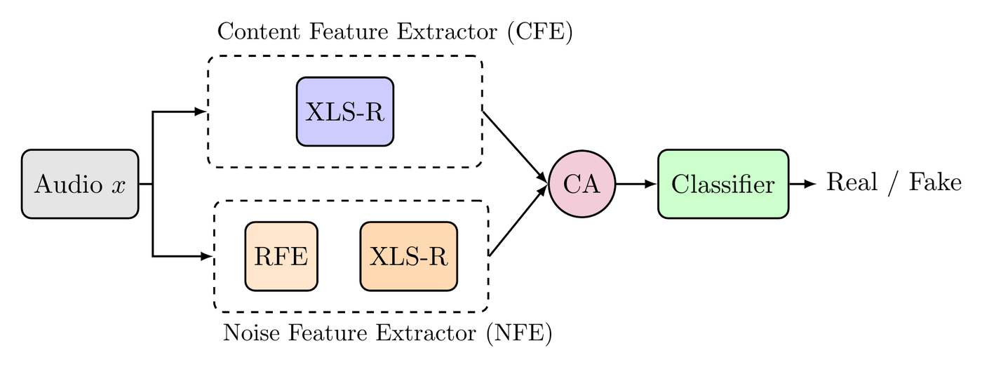
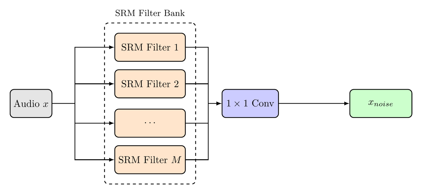
Architecture
Headline results
EER (%, lower is better) under a strict single-run protocol — no checkpoint averaging, no ensembling. Bold is the best per column.
| Model | DF EER ↓ | LA EER ↓ | In-the-Wild EER ↓ |
|---|---|---|---|
| XLSR + AASIST (baseline) | 3.69 | 1.90 | 10.46 |
| XLSR-Mamba | 1.88 | 0.93 | 6.71 |
| SONAR-Full | 1.57 | 1.55 | 6.00 |
| SONAR-Finetune | 1.45 | 1.20 | 5.43 |
XLSR-Mamba retains the lead on the in-domain LA partition (it was trained with checkpoint averaging on multiple seeds); SONAR is strongest where it matters most for deployment — out-of-distribution detection (DF and In-the-Wild).
Key findings
- Spectral bias is a generalisation bottleneck. When low-frequency content is removed (high-pass > 4 kHz), baseline models collapse to 32% EER while SONAR retains 26% — direct evidence the baseline relies on LF correlations, while SONAR captures genuine HF artifacts.
- The gain is alignment, not capacity. A dual-encoder model without RFE or JS scores 8.91% on ITW; full SONAR scores 6.00% with the same parameter count.
- 4× faster convergence. SONAR-Full stabilises in 12 epochs (Tak et al. trained 100); SONAR-Finetune in 4–6 epochs.
- Robust to codecs. Through MP3, Opus, Vorbis, and the DAC neural codec, score ranking is preserved (Spearman ρ = 0.944 for DAC).
- 2× FLOPs, 2× params, but only ~25% wall-clock overhead because the two encoders run concurrently on GPU (29 ms → 57 ms / 4-s clip).
- SONAR's noise branch carries the HF discriminative load. See Figure 3 below.
Where the HF signal lives inside SONAR
SONAR's central claim is that audio deepfake detectors miss high-frequency artifacts because the encoder itself is HF-blind. To test that claim directly — and to ask whether SONAR's training fixes the blindness — we run a simple probing experiment on the trained encoders.
Setup. We freeze the encoder, take each clip, high-pass filter it at fc = 4 kHz (everything below 4 kHz removed), feed it through the encoder, and mean-pool the resulting sequence into a single fixed-length embedding. We then train a small linear classifier on those embeddings to distinguish real from fake on the In-the-Wild test set. If the encoder genuinely carries HF cues, the linear probe will discriminate well; if the encoder discards HF information, the probe will be near chance.
What we vary. We compare three encoders and sweep how much training data the probe sees (10%, 25%, 50%, 100% of the dev set). More data should help if the HF signal exists in the embedding but is faint and hard to extract from few samples.
- Baseline XLSR — the off-the-shelf, single-encoder XLSR + AASIST detector (red, dashed).
- SONAR content branch — one of SONAR's two SSL encoders; sees the raw waveform like the baseline (green).
- SONAR noise branch — the other SSL encoder; receives SRM-filtered audio and is JS-aligned with the content branch during training (blue).
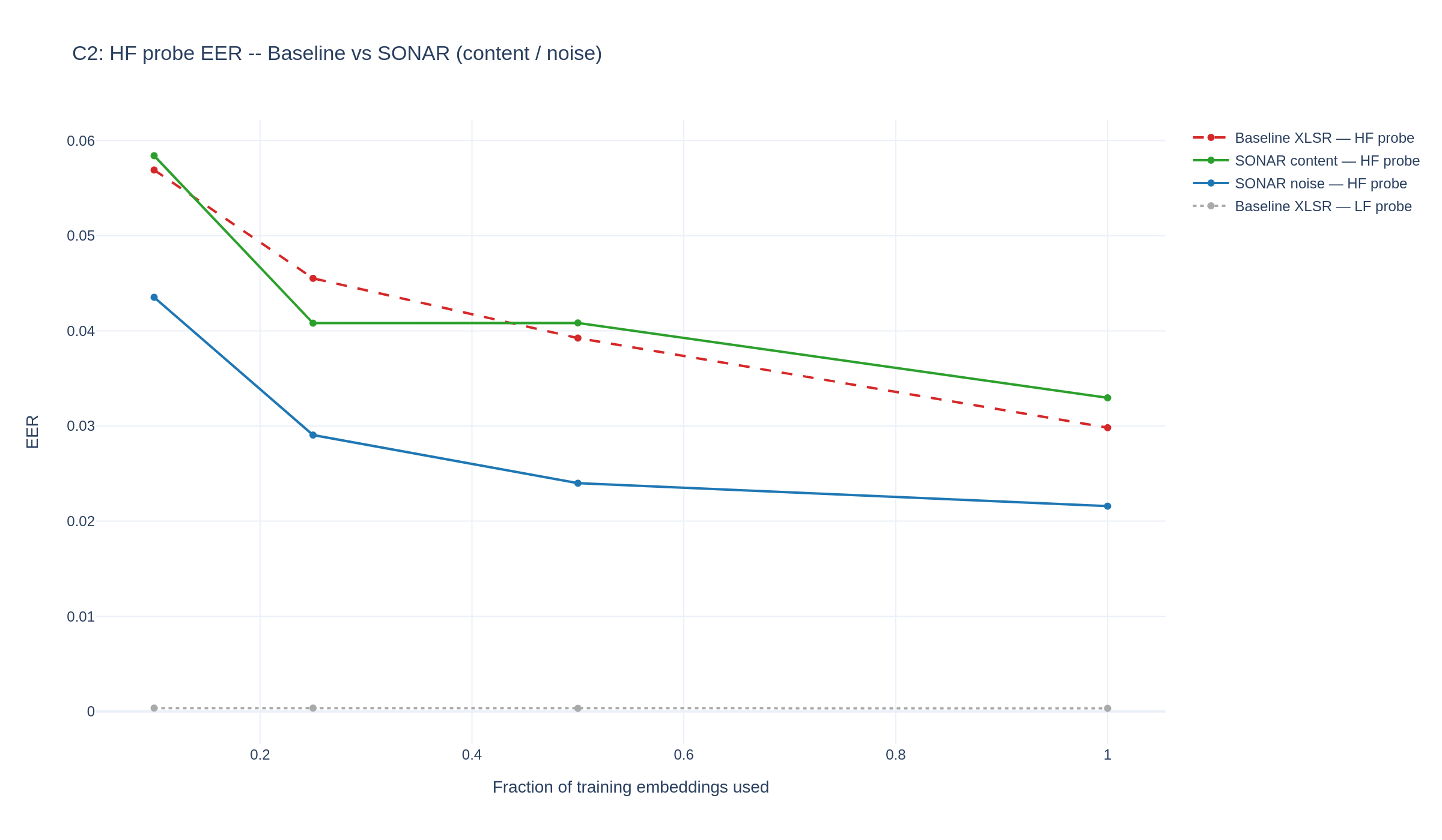
Two findings.
- The SONAR noise branch is decisively less HF-blind than the baseline at every training fraction. At full data its HF-probe EER is 2.16% versus 2.98% for the baseline — a 28% relative reduction; at 10% data the gap is even larger (4.35% vs 5.69%, 24% relative).
- The SONAR content branch sits roughly on top of the baseline. SONAR does not retrain the content encoder out of its spectral bias.
Reading these together. SONAR doesn't fix HF blindness inside the content encoder — it compensates for it architecturally, by allocating a parallel encoder to the HF residual and tying its distribution to the content distribution through the Jensen–Shannon alignment loss. The HF discriminative load that the baseline cannot carry ends up in SONAR's noise branch.
Citation
@inproceedings{hidekel2026sonar,
  title     = {{SONAR}: Spectral-Contrastive Audio Residuals for Generalizable Deepfake Detection},
  author    = {Hidekel, Ido Nitzan and Lifshitz, Gal and Cohen, Khen and Raviv, Dan},
  booktitle = {Proceedings of the 43rd International Conference on Machine Learning (ICML)},
  year      = {2026}
}